We are going to take a different way of learning. Here I’m presenting question answer based method in which I’ll show the code first and ask questions about it. This is similar to real-world learning where we do something and keep asking ourselves questions until we understand it properly.

Here’s the table of contents:

1. What is Contrastive Loss?
2. Why MNIST Data?
3. Basic Setup
4. Creating Dataset
   1. Code for creating dataset objects for train and validation
   2. Code for MNIST dataset class
5. DataLoaders
6. Model
7. Our Loss Function
8. Training Model
9. Infrencing
10. Why Cosine similarity?
11. Getting Embedding
    1. Getting Embedding of Train Data:
12. Why and How Annoy?
13. Inferencing
14. Getting Model Accuracy
15. Visualising Embeddings

What is Contrastive Loss?

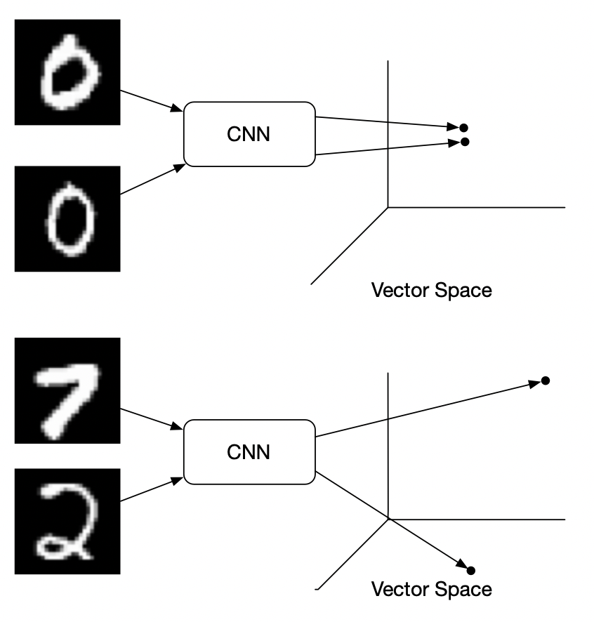
Contrastive loss is used in a classification task. It says that in embedding space same class vectors should be near and different class vectors should be apart. It is regarded as an alternative to Cross-Entropy loss.

The contrastive loss function computes the distance between pairs of examples in the embedding space and then applies a penalty if the distance is greater than a certain threshold. Specifically, for a given pair of examples, the contrastive loss function calculates the Euclidean distance between their embedding vectors. If the distance is below a certain threshold, a small loss is incurred; if it is above the threshold, a larger loss is incurred. The idea is to encourage the model to learn embeddings that make similar examples closer together and dissimilar examples further apart.

Why MNIST Data?

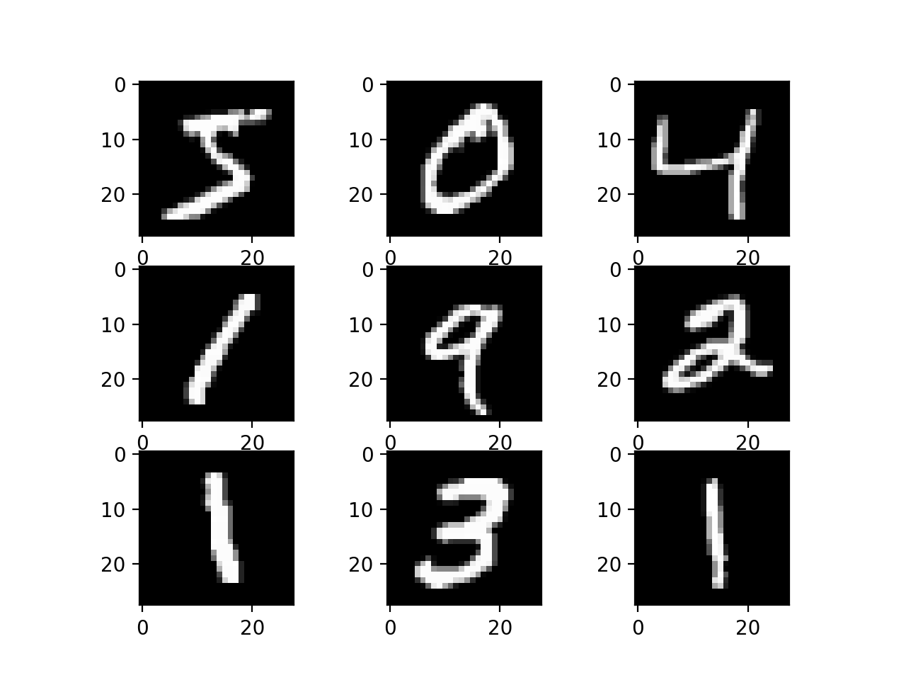
MNIST is a large collection of handwritten digit images. It has 10 class labelling i.e. zero to nine. Images are black and white with 28 * 28 fixed size. The simplisity of this dataset makes it ideal for learners to do image classification.

Basic Setup

We won’t be using many pre-built functions. As we are learners we’ll build our own model and dataset class. We’ll be using Pytorch. Also as Pytorch doesn’t have a contrastive loss function we’ll build it ourselves. let’s start with basic imports

import torch
import numpy as np
import pandas as pd
from torch import nn, optim
from torch.utils.data import Dataset, DataLoader
from torchvision import transforms
import matplotlib.pyplot as plt
from annoy import AnnoyIndex
import torchvision
from tqdm.notebook import tqdm

We’ll talk about Annoy in the later part of the post. We are using torch-vision to perform image tasks like transforms and resizing. Matplotlib is used for plotting and Tqdm is for showing the progress bar.

Creating Dataset

We’ll extend Pytorch class Dataset to create MNIST dataset class. There are 3 important functions of the class.

1. __init__ method: It is the initializer of the class. We can pass toggles and data to the class and change behaviour on it. We’ll use this method to do all the post-processing on the data.
2. __len__ method: This returns the lenth of the dataset.
3. __getitem__ method: This returns ith item from the dataset. This method can be used to do runtime data creation. But here we’ll keep data prepared to save time on training.

Let’s jump on the code for Dataset. Just read it once and create questions. we’ll get answers one by one

Code for creating dataset objects for train and validation

We have a dataset class MNISTDataset and we’ll use it to create train_dataset and val_dataset. Given that our input data is randomly arranged we’ll split the dataframe into two with 1000 records in the validation set and the rest in the train. We are using image transform to convert data into PIL Image -> Torch Tensors -> Normalized data.

# load data from csv
data = pd.read_csv('/kaggle/input/digit-recognizer/train.csv')
val_count = 1000
# common transformation for both val and train
default_transform = transforms.Compose([
    transforms.ToPILImage(),
    transforms.ToTensor(),
    transforms.Normalize(0.5, 0.5)
])
# split data into val and train
dataset = MNISTDataset(data.iloc[:-val_count], default_transform)
val_dataset = MNISTDataset(data.iloc[-val_count:], default_transform)

Code for MNIST dataset class

The code defines a PyTorch dataset class called MNISTDataset that is used for loading and processing MNIST data in the desired format. The MNISTDataset class takes a Pandas DataFrame containing MNIST data as input, along with an optional data transformation function and a boolean flag is_test indicating whether the data is being used for testing or training.

The MNISTDataset class randomly selects pairs of images from the input data for training, with each pair consisting of a “positive” example (an image with the same label as the current image) and a “negative” example (an image with a different label than the current image). For each row, the dataset class returns the two images, a label indicating whether they are positive or negative examples (doing it randomly), and the label of the original image. The second image is chosen randomly and whether the second image is of the same class or not is also random having 50-50 chances. This ensures that the dataset returns 50% positive pairs and 50% negative pairs.

If is_test is True, the dataset class will not generate positive or negative examples, and will instead return a single image with a label of -1.

The len method returns the total number of samples in the dataset and the getitem method returns a single sample from the dataset as a tuple of the two images, the label indicating whether they are positive or negative examples, and the label of the original image. The data is also transformed if a transformation function is provided.

This implementation is used for Siamese Neural Networks that are trained with Contrastive Loss to learn a metric space where similar examples are closer to each other and dissimilar examples are further apart.;

class MNISTDataset(Dataset):
    def __init__(self, data_df: pd.DataFrame, transform=None, is_test=False):
        # method will run once when class object is created.
        # method will create data at the time of object creation.
        # this will save time of training
        super(MNISTDataset, self).__init__()
        dataset = []
        labels_positive = {}
        labels_negative = {}
        if is_test == False:
            # for each label create a set of same label images.
            for i in list(data_df.label.unique()):
                labels_positive[i] = data_df[data_df.label == i].to_numpy()
            # for each label create a set of image of different label.
            for i in list(data_df.label.unique()):
                labels_negative[i] = data_df[data_df.label != i].to_numpy()

        for i, row in tqdm(data_df.iterrows(), total=len(data_df)):
            data = row.to_numpy()
            # if test then only image will be returned.
            if is_test:
                label = -1
                first = data.reshape(28, 28)
                second = -1
                dis = -1
            else:
                # label and image of the index for each row in df
                label = data[0]
                first = data[1:].reshape(28, 28)
                # probability of same label image == 0.5
                if np.random.randint(0, 2) == 0:
                    # randomly select same label image
                    second = labels_positive[label][
                        np.random.randint(0, len(labels_positive[label]))
                    ]
                else:
                    # randomly select different(negative) label 
                    second = labels_negative[label][
                        np.random.randint(0, len(labels_negative[label]))
                    ]
                # cosine is 1 for same and 0 for different label
                dis = 1.0 if second[0] == label else 0.0
                # reshape image
                second = second[1:].reshape(28, 28)

            # apply transform on both images
            if transform is not None:
                first = transform(first.astype(np.float32))
                if second is not -1:
                    second = transform(second.astype(np.float32))

            # append to dataset list. 
            # this random list is created once and used in every epoch
            dataset.append((first, second, dis, label))
        
        self.dataset = dataset
        self.transform = transform
        self.is_test = is_test

    def __len__(self):
        return len(self.dataset)

    def __getitem__(self, i):
        return self.dataset[i]

DataLoaders

The code defines two PyTorch DataLoader objects: trainLoader and valLoader. DataLoader is a PyTorch class that provides an efficient way to load data in batches during the training or evaluation of a model.

The batch_size argument sets the number of samples in each batch of data. The shuffle argument indicates whether to shuffle the data at the beginning of each epoch. The pin_memory argument is set to True, which enables faster data transfer to the GPU by allocating memory in pinned memory. The num_workers argument specifies the number of subprocesses to use for loading the data.

Here is the code

# create torch dataloader.
# shuffle true for train data to randomly create batches
trainLoader = DataLoader(
    dataset,
    batch_size=64,
    shuffle=True,
    pin_memory=True,
    num_workers=2,
    prefetch_factor=100
)
valLoader = DataLoader(val_dataset,
    batch_size=64,
    shuffle=True,
    pin_memory=True,
    num_workers=2,
    prefetch_factor=100
)

Model

class Network(nn.Module):
    def __init__(self):
        super(Network, self).__init__()
        self.conv1 = nn.Sequential(
            nn.Conv2d(1, 32, 5),
            nn.BatchNorm2d(32),
            nn.ReLU(inplace=True),
            nn.MaxPool2d((2, 2), stride=2),
            nn.Dropout(0.3)
        ) # d * 32 * 12 * 12
        self.conv2 = nn.Sequential(
            nn.Conv2d(32, 64, 5),
            nn.BatchNorm2d(64),
            nn.ReLU(inplace=True),
            nn.MaxPool2d((2, 2), stride=2),
            nn.Dropout(0.3)
        ) # d * 64 * 4 * 4
        self.linear1 = nn.Sequential(
            nn.Linear(64 * 4 * 4, 512),
            nn.ReLU(inplace=True),
            nn.Dropout(0.3),
            nn.Linear(512, 64),
        )

    def forward(self, x):
        x = self.conv1(x) # x: d * 32 * 12 * 12
        x = self.conv2(x) # x: d * 64 * 4  * 4 
        x = x.view(x.size(0), -1) # x: d * (64*4*4)
        x = self.linear1(x) # x: d * 64
        return x

This code defines a neural network architecture for image classification using PyTorch.

The class Network inherits from nn.Module, which is a base class for all neural network modules in PyTorch. It has two main components: a convolutional layer and a fully connected layer.

The convolutional layer consists of two sequential layers of 2D convolutional neural networks with 32 and 64 output channels, respectively. Each convolutional layer is followed by batch normalization, ReLU activation function, max pooling, and dropout. The output of the first convolutional layer has a dimension of d * 32 * 12 * 12, where d is the batch size, while the output of the second convolutional layer has a dimension of d * 64 * 4 * 4.

The fully connected layer consists of two sequential linear transformations with ReLU activation function and dropout. The first linear transformation reduces the input from 64 * 4 * 4 to 512 dimensions, and the second linear transformation reduces it further to 64 dimensions.

The forward function defines how the input data flows through the network. First, the input data is passed through the convolutional layers. Then, the output is flattened to a one-dimensional tensor using the view function. Finally, the flattened tensor is passed through the fully connected layer to produce the final output.

Our Loss Function

class ContrastiveLoss(nn.Module):
    def __init__(self):
        super(ContrastiveLoss, self).__init__()
        self.similarity = nn.CosineSimilarity(dim=-1, eps=1e-7)

    def forward(self, first, second, distance):
        # use cosine similarity from torch to get score
        score = self.similarity(first, second)
        # after cosine apply MSE between distance and score
        return nn.MSELoss()(score, distance)

This code defines a custom loss function for a contrastive learning task

The class takes an argument m which represents a margin that separates the positive and negative pairs. The CosineSimilarity function from nn module is used to calculate the cosine similarity between the first and second inputs along the last dimension (-1) with a small epsilon value to avoid division by zero.

The output of the forward function is a scalar loss value that measures how well the model is performing on the contrastive task. The loss is calculated based on how close the similarity score between the inputs is to the ground truth similarity score. If the similarity score is close to the ground truth similarity score, the loss will be low. Conversely, if the similarity score is far from the ground truth similarity score, the loss will be high. The loss function encourages the model to learn representations of the inputs that capture their similarity.

Training Model

# define optimizer
optimizer = optim.Adam(net.parameters(), lr=0.001)
# define loss function
loss_function = ContrastiveLoss()
# define learning rate scheduler
scheduler = optim.lr_scheduler.StepLR(optimizer, step_size=7, gamma=0.3)

Here we create an optimizer and a learning rate scheduler

lrs = []
losses = []
# torch training loop
for epoch in range(50):
    epoch_loss = 0
    batches=0
    print('epoch -', epoch)
    lrs.append(optimizer.param_groups[0]['lr'])
    print('learning rate', lrs[-1])
    for first, second, dis, label in tqdm(trainLoader):
        batches+=1
        optimizer.zero_grad()
        first_out = net(first.to(device))
        second_out = net(second.to(device))
        dis = dis.to(torch.float32).to(device)
        loss = loss_function(first_out, second_out, dis)
        epoch_loss+=loss
        loss.backward()
        optimizer.step()
    # append epoch loss for plotting
    losses.append(epoch_loss.cpu().detach().numpy()/batches)
    # scheduler step at every epoch
    scheduler.step()
    print('epoch_loss', losses[-1])

Here we loop for 50 epochs and train our model with the loss function we created.

Infrencing

This is where we make our app production ready and test the accuracies. Since our model only gives embedding and doesn’t share classes we have to find another way. We have to have an algorithm which can find the nearest embedding for the given embedding. Also, we have to create a database of all train images with embeddings to check which is the nearest to predict. Fortunately, these things have been incorporated into a library Annoy which is very fast and reliable. We’ll fetch N nearest samples and check which class have the most contribution in it. That’ll be our prediction.

Why Cosine similarity?

Embedding is a multi-space vector. Our imagination cannot go beyond 3D but we can use maths to form an idea of it. For example, in 3D or 2D we can get the distance between two points which is called the Euclidean distance of vector. We can also find the angle between both this is cosine distance. The less these distances are the more similar vectors are or the more near points arr.

Now, why do we choose Cosine over Euclidean?

We are using a lot of dimensions and each dimension value is between 0 - 1. In these settings, Cosine tends to work better than Euclidean because cosine ignores the length of the vectors and only sees the angular difference. So if two points are in the same line then Cosine < Euclidean.

Getting Embedding

What is embedding?? embedding refers to the process of representing entitye (word, phrases or image) in a numerical form that can be used by machine learning algorithms for various tasks, such as text classification, sentiment analysis, and machine translation.

The process involves mapping each word or phrase to a high-dimensional vector of real numbers, often referred to as an embedding vector or simply embedding. We can say it is a array of size N which describes the image.

Getting Embedding of Train Data:

Why train data?? Since our model gives only embedding and not label, So we’ll index (keep) train data and use it to get predictions.

code to get embedding of train data:

outputs = []
labels = []
net.eval()
# loop over train data and get embedding for each image
with torch.no_grad():
    for first, second, dis, label in tqdm(trainLoader):
        outputs.append(net(first.to(device)).cpu().detach().numpy())
        labels.append(label.numpy())

# np.concatenate to convert list into np.array
outputs = np.concatenate(outputs)
labels = np.concatenate(labels)

Why and How Annoy?

Annoy uses a tree-based algorithm and splits data at every level in N-Dimensional space. It uses a straight line to split data. This made it fast to get the nearest samples from conventional Algos which compare every point pair. Annoy is not fully accurate from conventional algorithms but it is very fast. To improve accuracy annoy creates a forest [ K number of trees ] and gives an ensembled result.

code to index data in annoy:

from annoy import AnnoyIndex
# create an annoy forest, add train data and save
forest = AnnoyIndex(outputs.shape[1], metric='angular')
for i, item in tqdm(enumerate(outputs)):
    forest.add_item(i, item)
forest_labels = labels
forest.build(10)
forest.save('/kaggle/working/forest.ann')

Here we are building forest of 10 trees. The move trees we create the better and accuracy of nearest image will be. But I’ll take more disk space when we save it and more memory when we load it. Also, We are using angular as metric which tells Annoy to use angular distance to compare items.

Inferencing

Now that we have out Annoy build we’ll use it for predictions. below is a small function to get prediction for an image.

from scipy import stats
def inferance(forest, forest_labels, image):
    net.eval()
    with torch.no_grad():
        test_outs = net(image.to(device))
    labels=[]
    for i in test_outs:
        # get 10 nearest images for given image
        indexes = forest.get_nns_by_vector(i.cpu().detach().numpy(), 10)
        # get mode label of the 10 images. 
        # other methods can be used here
        labels.append(stats.mode(forest_labels[indexes])[0][0])
    return np.array(labels)

Note: Model it set to eval model so that dropout is inactive. Otherwise it’ll give unwanted results

In above code we got embedding from model for the image and then got 10 nearesh neighbors by using forest.get_nns_by_vector. We have labels for these 10 neighbors so we take mode of it.

Getting Model Accuracy

We’ll use our inference method to get models accuracy on Eval data. below is the code

acc = []
count = 0
y_eval, eval_results = [], []
# for every val data get inference output and calculate accuracy
for image, _, _, image_labels in tqdm(evalLoader):
    count+=1
    results = inferance(forest, labels, image)
    y_eval.append(image_labels.numpy())
    eval_results.append(results[:len(image_labels.numpy())])
    acc.append((results[:len(image_labels.numpy())] == image_labels.numpy()).mean())
print('Eval Accuracy', statistics.mean(acc))

For me output is Eval Accuracy 0.9912109375

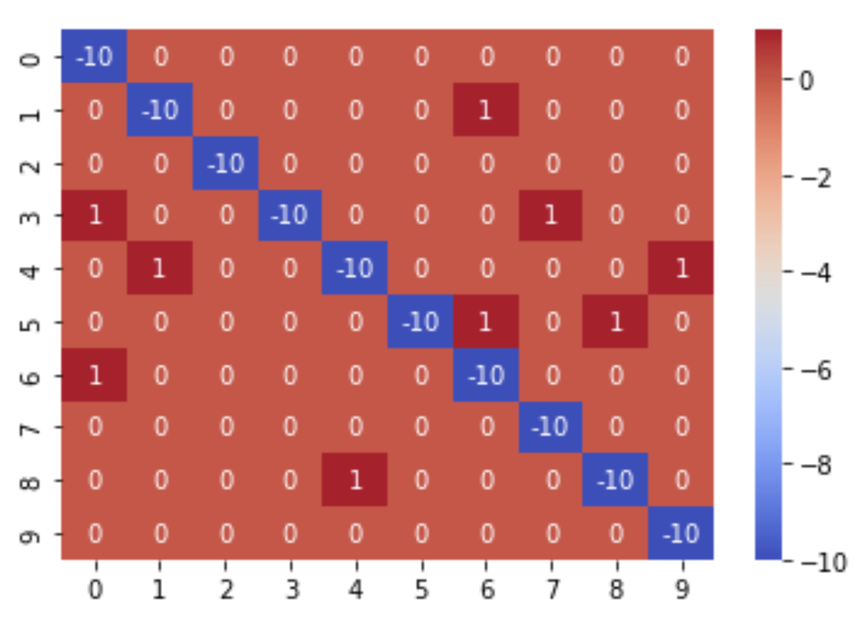
We’ll also print confusion matrix for eval data. below is the code

import seaborn as sns
from sklearn.metrics import confusion_matrix

# plot confusion metrix using sklearn.metrics.confusion_matrix
conf_m = confusion_matrix(np.concatenate(y_eval), np.concatenate(eval_results))
conf_m[[range(0, len(conf_m)), range(0, len(conf_m))]] = -10
sns.heatmap(conf_m, annot=True, fmt='g', cmap='coolwarm')

we’ll get output:

Visualising Embeddings

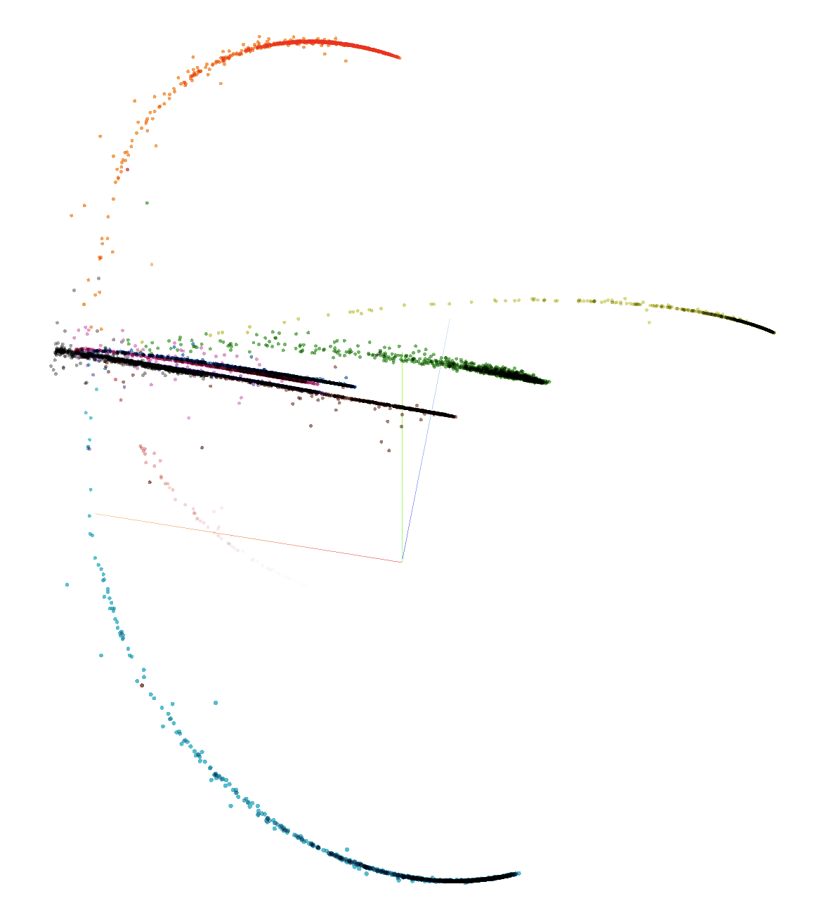
Visualising more than 3D is hard for humans. Our Model return embedding of size 64 which seems to be impossible to visualize currenly. There are few method which can be used to bring higher dimentions data into lower dimentions. One way is to use PCA (Principle Component Analysis).

Above is PCA of train data in 3D. We can see that embeddings are saperated by labels which verify that our model is giving distance to non similar embeddings. To verify open link (in color by select labels)